The efficiency of hydraulic systems is a key topic in which the reduction of dissipation plays a fundamental role in its increase: for this reason it is often important to optimize or, in any case, to be aware of the pressure drops existing in a circuit during an operating cycle. The consequences of high pressure drops are from an increase in the pressure level in the system, to the additional generation of heat to be removed (thus requiring additional energy). The main losses come from the hydraulic pumps, motors and valves that drive the actuators but a significant improvement in their reduction can be obtained by optimizing the fluid paths in the pipes and manifolds.
There are several ways to know the pressure drops in a path:
- Test on the test bench of the real circuit
- CFD simulations using the 3D design of the path
- Calculation with theoretical formulas
As you can guess, the 3 solutions are in increasing order of simplicity of calculation but decreasing of accuracy. SmartFluidPower has created a design tool that allows you to very quickly estimate the pressure drops in a hydraulic circuit, looking for a compromise between accuracy and difficulty in obtaining the result.
The procedure consists in setting the boundary conditions (properties of the fluid and its flow rate) and entering the characteristics of all the occurrences that the fluid encounters from the inlet to the outlet: section contractions/expansions, elbows, straight ducts, orifices, known concentrated pressure drops (valves, etc.). The tools uses semi-empirical formulas to calculate the pressure drops in each of the inserted geometries. The result is a sum of all the values and, of course, it is immediate to recalculate it by changing the conditions of the fluid or geometric characteristics of the various ‘blocks’ inserted.
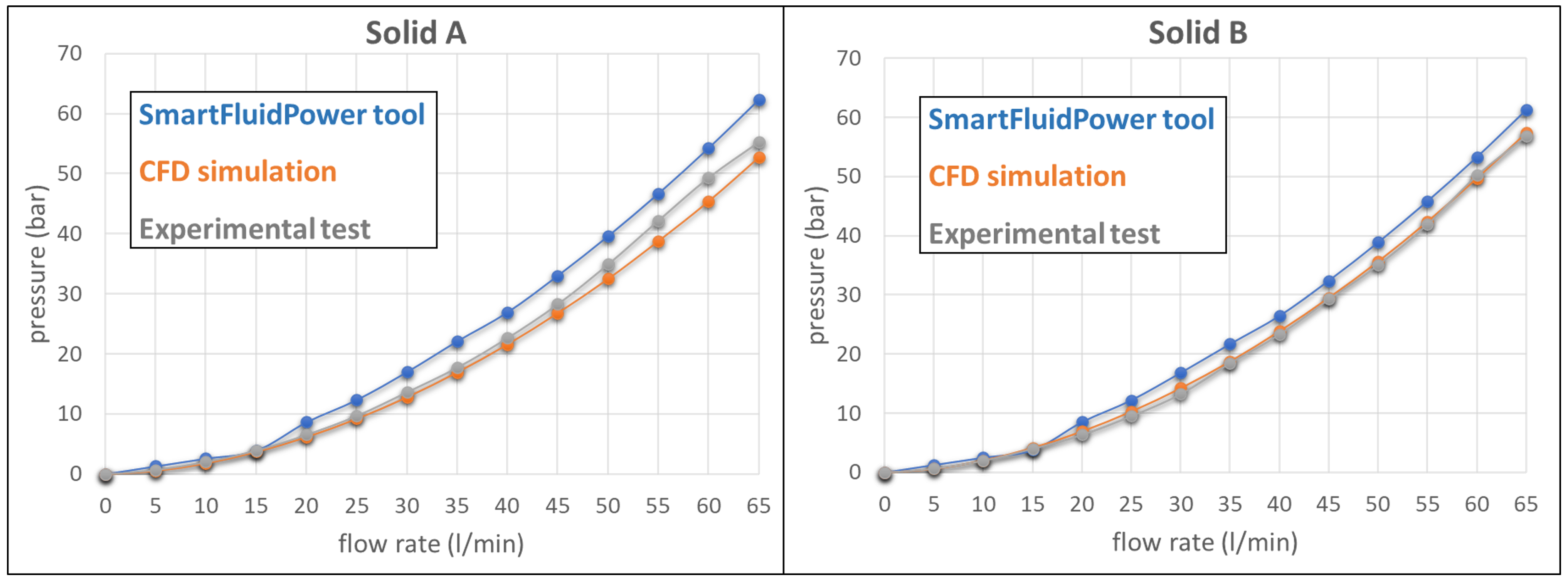
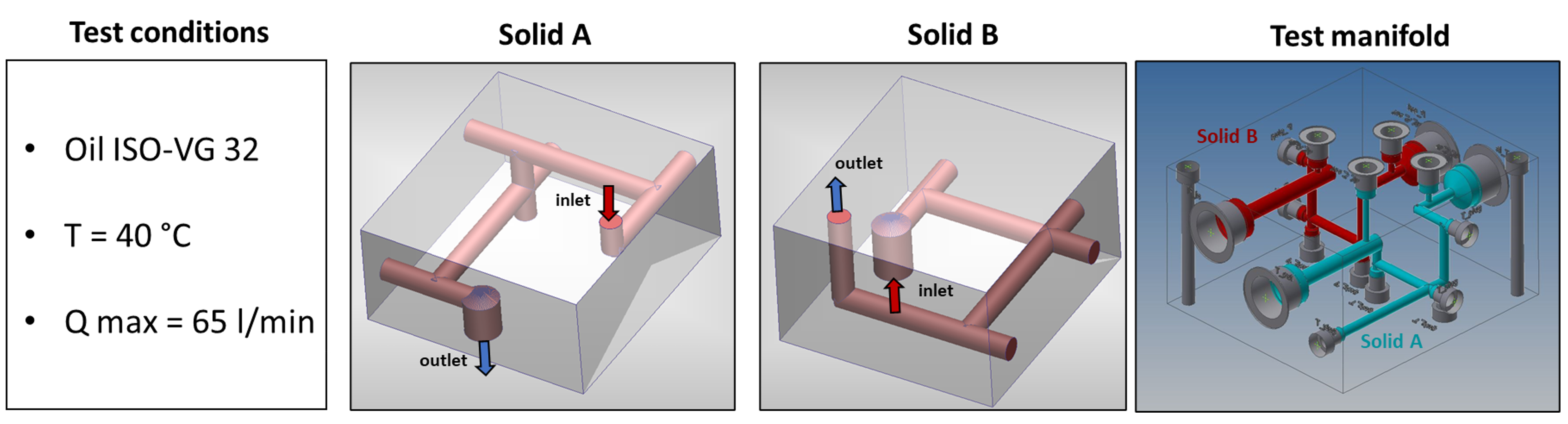
The two example paths on which the pressure drops are calculated are shown below: the results are also compared experimentally by making the two paths in a manifold and testing them on the test bench.
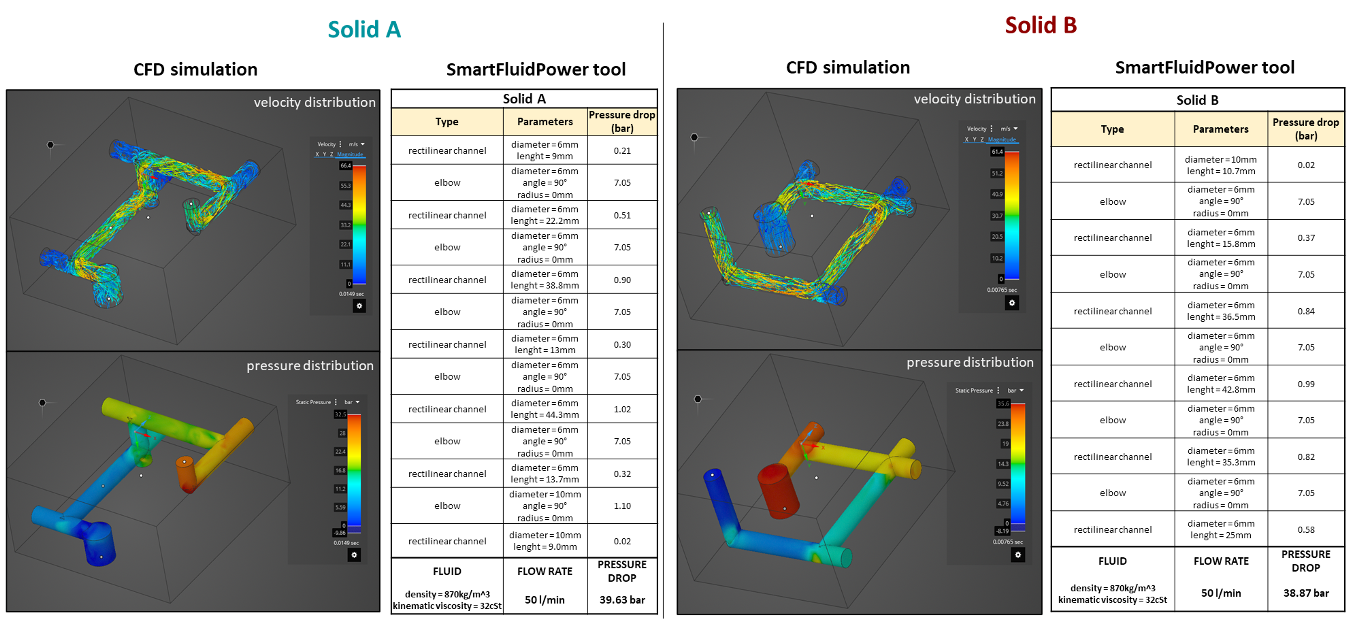
The figure shows the two software tools for calculating pressure drops: the CFD simulations with the velocity and pressure distributions and the SmartFluidPower tool with the list of ‘obstacles’ encountered by the fluid along the way.
The graphs summarize the pressure drop results as a function of the flow rate, obtained for the two paths and comparing the 3 methodologies. Taking the experimental data as a reference (even if always affected by a certain error), CFD simulations provide an average error of 6.6% in ‘Solid A’ and 3.1% in ‘Solid B’. The SmartFluidPower tool has a higher error (14.9% ‘Solid A’ and 12.5% ’Solid B’) always overestimating the reference value (therefore conservative), but gaining significantly in the speed and simplicity of calculating the curves.