How the new update changes the way fluid is described in fluid power simulations. A case study shows the library's flexibility in practice.

Why Viscosity and Density Are Not Just a Number
In fluid power system simulation, it is easy to treat fluid viscosity and density as two simple constants to enter into a parameter mask. In reality, both quantities vary significantly, primarily with temperature, but not only. Perhaps not everyone knows that the main properties of industrial oils also vary depending on operating pressure. Neglecting these dependencies leads to unreliable estimates of internal leakage, volumetric efficiency, or valve response times — precisely the quantities a simulation should help predict.
With version 4.0 of SFPLibDyn, we have expanded the core of the library’s fluid properties: the goal was to let those modeling the system choose the level of detail best suited to their case — from a simple constant up to a full model dependent on temperature and pressure — without having to touch the rest of the hydraulic circuit.
Want to see how viscosity changes with pressure, temperature, or fluid properties? With the interactive calculator at this link, you can set your own parameters (or start from a standard ISO VG configuration) and instantly view the resulting curve.
A “Composable” Fluid
In previous versions, the fluid properties were tied to a fixed calculation model that only considered the influence of temperature. Starting with this release, the calculation model describing the simulation fluid is modular and exposes two replaceable components:
- ViscModel_l — the liquid’s viscosity model
- DensityModel_l — the liquid’s density model
Each of the two components can be replaced directly from the FluidProp parameter window in the OpenModelica simulation environment. With just a few clicks, it becomes possible to compare the results of multiple simulations using different fluid models. The various selectable options offer different levels of accuracy and dependency — from the simplest, which keeps values constant, to the most complete, which accounts for every contribution of pressure and temperature.
This approach makes it straightforward to move from a simplified fluid during preliminary sizing to an accurate characterization during final validation, simply by changing two menu entries.
Case Study: How Much Does Choosing the Right Model Matter in Practice?
To make the effect of model choice concrete, let’s consider a typical case: an ISO VG46 hydraulic oil, in a system operating at a steady-state pressure of 350 bar, with fluid temperature rising from 40 °C at start-up to 80 °C once thermal steady state is reached (a common condition in the off-road sector, for example inside an axial piston pump or a throttling element).
Let’s compare three possible configurations of ViscModel_l for the same circuit:
| Model | Dependencies | Description |
|---|---|---|
| Constant | None | Viscosity is fixed at the nominal value (46 cSt) |
| ISO3448 | Temperature | Viscosity is corrected as a function of temperature only, via standard tables |
| ISO3448Extended | Temperature and pressure | The viscosity obtained from the tables is corrected using an exponential relationship with the sensitivity coefficient λₚ (value used: λₚ = 450 bar) |
| Operating condition | Constant | ISO3448 | ISO3448Extended |
|---|---|---|---|
| Start-up — 40 °C, 50 bar | 46 cSt (by definition) | ≈ 46 cSt (standard ISO VG 46 value at 40 °C) | ≈ 46 × exp(50/450) ≈ 51.5 cSt |
| Steady state — 80 °C, 350 bar | 46 cSt (no variation) | ≈ 11.9 cSt (typical ISO VG 46 value at 80 °C) | ≈ 11.9 × exp(350/450) ≈ 25.9 cSt |
The resulting figure is significant: at steady-state conditions, the Constant model overestimates the actual viscosity by more than double compared to the T+p estimate, while the ISO3448 model (which considers temperature only) underestimates it by more than half, because it ignores the stiffening effect of pressure. Only the ISO3448Extended model captures the balance between the two opposing effects (thinning due to temperature, stiffening due to pressure).
In terms of performance, this translates as follows: since leakage through a laminar clearance is, to a first approximation, inversely proportional to viscosity, a model that ignores the pressure dependence can overestimate internal leakage (and therefore underestimate volumetric efficiency) by as much as a factor of two, at the same operating condition. A model that ignores temperature and pressure dependence altogether, on the other hand, risks the opposite error: underestimating leakage and heat generation during the hot phases of the cycle.
Available Models
The library provides three formulations, designed to cover both the simplest cases and characterization based on technical data sheet values typical of the fluid power and petroleum industries. Library users are free to decide which calculation model best suits their needs.
Below is an overview of the available models and their main characteristics. A complete description of each model and the required parameters is available in the library documentation.
| Model | T | p | When to use it |
|---|---|---|---|
| Density | |||
| Constant | ❌ | ✅* | If you want to use a precise viscosity value |
| GeneralExpansionCoeff | ✅ | ✅* | Mineral oils with a known expansion coefficient |
| VCF | ✅ | ✅* | Follows the standards most widely used in the oil industry, so the data reported on suppliers' technical data sheets can be used directly |
| Viscosity | |||
| Constant | ❌ | ❌ | If you want to use a precise viscosity value |
| ISO3448 | ✅ | ✅ | ISO VG class, for applications with controlled pressure values |
| ISO3448Extended | ✅ | ✅ | If you want to use a standard oil for high-pressure applications |
| LambdaExtended | ✅ | ✅ | Fully characterized fluid, if the sensitivity terms λₚ and λT are known (or experimental results are available for 3 distinct conditions) |
* The pressure dependence of density is always present, regardless of the selected model. All models require the bulk modulus, used by the library's equations to describe the fluid's compressibility. Density models act exclusively on the variation with temperature.
In Summary
The 4.0 update introduces a modular approach to describing fluid in SFPLibDyn: independently for density and viscosity, users can choose the most suitable trade-off between simplicity and physical accuracy, from a constant up to the full model dependent on temperature and pressure.
The benefit is not limited to mineral oils: the same architecture applies to any liquid — water, fuels, biodegradable fluids, or other industrial fluids — simply by parameterizing the chosen model with the available data, whether it be an ISO class, a supplier’s technical data sheet, or laboratory measurements.
For the designer, this means being able to increase simulation realism without increasing model complexity — reducing the risk of surprises when moving from the model to the test bench.
Want to Learn More?
If you would like to explore how to integrate these models into your simulations, or would like a demonstration of the library, get in touch: we would be happy to show you how to use SFPLibDyn in your specific application.