Trial version

Thank you for downloading the Trial version

The Trial version is a reduced version of the SFPLibDyn library developed specifically to allow you to test the simulation environment.

This section allows anyone who owns the Trial Library to navigate through all the functionalities maintained in this version.

Environment Preparation

1. First, make sure you have the system requirements, then install the version of OpenModelica that was provided to you along with the library (SFPLibDyn.mol).
2. To orient yourself within the software, we recommend reading the Quick Guide to OpenModelica section.

Specific Examples

Having a limited selection of components, it is not possible to test the example files provided in the specific section, therefore in this section some examples are proposed to download and use.

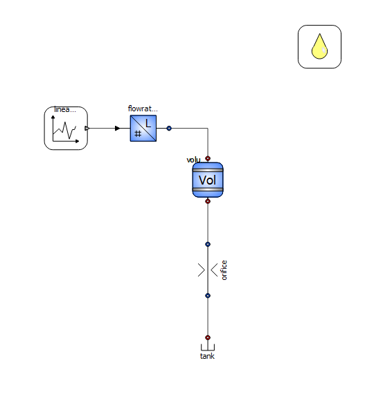
Example 1: flow rate-pressure curve through a throttle

Show the model or download it

model ex_1
SFPLibDyn.Hydraulic.Sources.FlowrateSource flowrateSource annotation(
    Placement(transformation(origin = {-20, 32}, extent = {{-12, -10}, {12, 10}})));
SFPLibDyn.Hydraulic.Sources.Tank tank annotation(
    Placement(transformation(origin = {10, -70}, extent = {{-6, -4.5}, {6, 4.5}})));
SFPLibDyn.Signals.Source.LinearStages linearStages(stage1_end = 60, stage1_duration = 0.5, stage2_duration = 0.5) annotation(
    Placement(transformation(origin = {-56, 32}, extent = {{-10, -10}, {10, 10}})));
inner SFPLibDyn.Properties.Hydraulic.FluidProp fluidProp annotation(
    Placement(transformation(origin = {62, 70}, extent = {{-10, -10}, {10, 10}})));
SFPLibDyn.Hydraulic.Volumes.Volume2p volume2p(vol_0 = 0.001, pressure(start = 0)) annotation(
    Placement(transformation(origin = {10, 8}, extent = {{-10, -10}, {10, 10}})));
SFPLibDyn.Hydraulic.Orifices.Orifice orifice annotation(
    Placement(transformation(origin = {10, -34}, extent = {{-6, -12}, {6, 12}})));
equation
connect(linearStages.y1, flowrateSource.u1) annotation(
    Line(points = {{-46, 32}, {-32, 32}}));
connect(flowrateSource.h1, volume2p.h2) annotation(
    Line(points = {{-8, 32}, {10, 32}, {10, 18}}));
connect(volume2p.h1, orifice.h2) annotation(
    Line(points = {{10, -2}, {10, -22}}));
connect(orifice.h1, tank.h1) annotation(
    Line(points = {{10, -46}, {10, -66}}));
annotation(
    uses(SFPLibDyn(version = "3.2")),
    __OpenModelica_simulationFlags(lv = "LOG_STDOUT,LOG_ASSERT,LOG_STATS", s = "dassl", variableFilter = ".*"),
    experiment(StartTime = 0, StopTime = 1, Tolerance = 1e-08, Interval = 0.002));
end ex_1;

In this exercise, a throttle is proposed that is traversed by an increasing then decreasing flow rate ramp. This scheme contains the basic elements that constitute our library:

• a capacitive element: the volume, which computes the internal pressure through the total balance of fluid it contains;
• a resistive element: the throttle, which processes a volumetric flow rate of fluid (exiting from the volume) that passes through the throttle as a function of the pressure drop acting on the element.

Consult the specific section for further details.

By double-clicking on the components, it is possible to change their properties: for example in the throttle through or_model it is possible to indicate which parameter to use to calculate the throttle size.

• Diameter: requires you to directly enter the hole diameter in the Diameter tab
• PQChar: requires the flow rate and pressure values characteristic of any point on its characteristic curve (to be entered in the PQChar tab). Through these two values the model processes the equivalent opening and therefore the instantaneous flow rate.

In the graphs section it is possible to create a parametric plot and visualize the resulting characteristic curve of the set throttle. For volumetric flow rates larger than those shown, adjust the parameters of linearStage of the signal source.

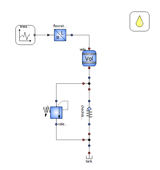
Example 2: relief valve and check valve in parallel

Show the model or download it

model ex_2
SFPLibDyn.Hydraulic.Sources.FlowrateSource flowrateSource annotation(
    Placement(transformation(origin = {-20, 56}, extent = {{-12, -10}, {12, 10}})));
SFPLibDyn.Hydraulic.Sources.Tank tank annotation(
    Placement(transformation(origin = {10, -70}, extent = {{-6, -4.5}, {6, 4.5}})));
SFPLibDyn.Signals.Source.LinearStages linearStages(stage1_end = 200, stage1_duration = 10)  annotation(
    Placement(transformation(origin = {-56, 56}, extent = {{-10, -10}, {10, 10}})));
inner SFPLibDyn.Properties.Hydraulic.FluidProp fluidProp annotation(
    Placement(transformation(origin = {62, 70}, extent = {{-10, -10}, {10, 10}})));
SFPLibDyn.Hydraulic.Valves.ReliefValve reliefValve(p_crack = 1.5e7, saturation = true, p_ch = 2.5e6, q_ch = 0.0033333333333333335)  annotation(
    Placement(transformation(origin = {-24, -24}, extent = {{-12, -12}, {12, 12}}, rotation = 180)));
SFPLibDyn.Hydraulic.Nodes.Node3p node3p annotation(
    Placement(transformation(origin = {10, -52}, extent = {{6, -6}, {-6, 6}}, rotation = -0)));
SFPLibDyn.Hydraulic.Valves.CheckValve checkValve(saturation = true, linear_parameter = SFPLibDyn.Units.Choices.InputType.q_sat, q_sat = 4.166666666666667e-4, p_ch = 1.5e6, q_ch = 4.166666666666667e-4)  annotation(
    Placement(transformation(origin = {10, -24}, extent = {{-6, -12}, {6, 12}}, rotation = 180)));
SFPLibDyn.Hydraulic.Nodes.Node3p node3p1 annotation(
    Placement(transformation(origin = {10, 6}, extent = {{6, 6}, {-6, -6}}, rotation = -0)));
SFPLibDyn.Hydraulic.Volumes.Volume2p volume2p(vol_0 = 0.001, pressure(start = 0))  annotation(
    Placement(transformation(origin = {10, 32}, extent = {{-10, -10}, {10, 10}})));
equation
connect(linearStages.y1, flowrateSource.u1) annotation(
    Line(points = {{-46, 56}, {-32, 56}}));
connect(node3p.h1, tank.h1) annotation(
    Line(points = {{10, -58}, {10, -66}}));
connect(node3p.h3, reliefValve.h2) annotation(
    Line(points = {{4, -52}, {-24, -52}, {-24, -36}}));
connect(node3p1.h2, checkValve.h1) annotation(
    Line(points = {{10, 0}, {10, -12}}));
connect(checkValve.h2, node3p.h2) annotation(
    Line(points = {{10, -36}, {10, -46}}));
connect(node3p1.h3, reliefValve.h1) annotation(
    Line(points = {{4, 6}, {-24, 6}, {-24, -12}}));
connect(flowrateSource.h1, volume2p.h2) annotation(
    Line(points = {{-8, 56}, {10, 56}, {10, 42}}));
connect(volume2p.h1, node3p1.h1) annotation(
    Line(points = {{10, 22}, {10, 12}}));
annotation(
    uses(SFPLibDyn(version = "3.2")),
__OpenModelica_simulationFlags(lv = "LOG_STDOUT,LOG_ASSERT,LOG_STATS", s = "dassl", variableFilter = ".*"),
experiment(StartTime = 0, StopTime = 10, Tolerance = 1e-08, Interval = 0.002));
end ex_2;

In this exercise it is possible to study the parameterization and behavior of a relief valve and a check valve. The pressure trend in the chamber will be highly influenced by the settings of these two valves.

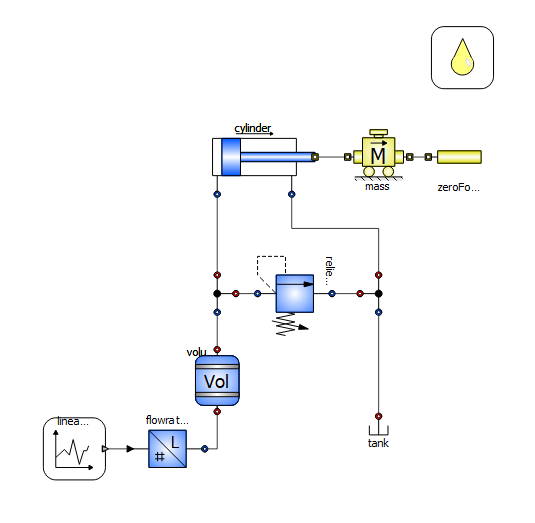
Example 3: control of a single-acting cylinder

Show the model or download it

model ex_3
SFPLibDyn.Hydraulic.Sources.FlowrateSource flowrateSource annotation(
    Placement(transformation(origin = {-33, -56}, extent = {{-12, -10}, {12, 10}})));
SFPLibDyn.Signals.Source.LinearStages linearStages(stage1_end = 120, stage1_duration = 0.2, stage2_end = 120, stage2_duration = 4.6, stage3_end = -120, stage3_duration = 0.4, stage4_end = -120, stage4_duration = 4.8) annotation(
    Placement(transformation(origin = {-63, -56}, extent = {{-10, -10}, {10, 10}})));
inner SFPLibDyn.Properties.Hydraulic.FluidProp fluidProp annotation(
    Placement(transformation(origin = {62, 70}, extent = {{-10, -10}, {10, 10}})));
SFPLibDyn.Hydraulic.Volumes.Volume2p volume2p(vol_0 = 0.003, pressure(start = 0)) annotation(
    Placement(transformation(origin = {-17, -34}, extent = {{-10, -10}, {10, 10}})));
SFPLibDyn.Mechanical.Translational.Mass mass(endstops_model = SFPLibDyn.Units.Choices.mass_type.Ideal, low_lim = 0, high_lim = 0.3, mass(displayUnit = "kg") = 3000, coeff_wind = 2e7) annotation(
    Placement(transformation(origin = {35, 38}, extent = {{-10, -10}, {10, 10}})));
SFPLibDyn.Hydraulic.Actuators.Cylinders.Cylinder cylinder(d_piston = 0.2, d_rod = 0.16, stroke = 0.3) annotation(
    Placement(transformation(origin = {-4, 37}, extent = {{-18.5, -11}, {18.5, 11}})));
SFPLibDyn.Hydraulic.Sources.Tank tank annotation(
    Placement(transformation(origin = {35, -50}, extent = {{-6, -4.5}, {6, 4.5}})));
SFPLibDyn.Hydraulic.Valves.ReliefValve reliefValve(p_crack = 4.5e6) annotation(
    Placement(transformation(origin = {8, -6}, extent = {{-12, -12}, {12, 12}}, rotation = -90)));
SFPLibDyn.Hydraulic.Nodes.Node3p node3p annotation(
    Placement(transformation(origin = {-17, -6}, extent = {{-6, -6}, {6, 6}})));
SFPLibDyn.Hydraulic.Nodes.Node3p node3p1 annotation(
    Placement(transformation(origin = {35, -6}, extent = {{6, -6}, {-6, 6}}, rotation = -0)));
SFPLibDyn.Mechanical.Translational.Sources.ZeroForce zeroForce annotation(
    Placement(transformation(origin = {61, 38}, extent = {{10, -10}, {-10, 10}}, rotation = -0)));
equation
connect(linearStages.y1, flowrateSource.u1) annotation(
    Line(points = {{-53, -56}, {-45, -56}}));
connect(mass.t1, cylinder.t1) annotation(
    Line(points = {{25, 38}, {14.5, 38}}));
connect(flowrateSource.h1, volume2p.h1) annotation(
    Line(points = {{-21, -56}, {-17, -56}, {-17, -44}}));
connect(node3p.h1, volume2p.h2) annotation(
    Line(points = {{-17, -12}, {-17, -24}}));
connect(cylinder.h1, node3p.h2) annotation(
    Line(points = {{-17, 26}, {-17, 0}}));
connect(node3p.h3, reliefValve.h1) annotation(
    Line(points = {{-11, -6}, {-4, -6}}));
connect(node3p1.h3, reliefValve.h2) annotation(
    Line(points = {{29, -6}, {20, -6}}));
connect(cylinder.h2, node3p1.h2) annotation(
    Line(points = {{7, 26}, {7, 15}, {35, 15}, {35, 0}}));
connect(node3p1.h1, tank.h1) annotation(
    Line(points = {{35, -12}, {35, -45.5}}));
connect(zeroForce.t1, mass.t2) annotation(
    Line(points = {{51, 38}, {45, 38}}));
annotation(
    uses(SFPLibDyn(version = "3.2")),
    __OpenModelica_simulationFlags(lv = "LOG_STDOUT,LOG_ASSERT,LOG_STATS", s = "dassl", variableFilter = ".*"),
    experiment(StartTime = 0, StopTime = 10, Tolerance = 1e-08, Interval = 0.002),
    Diagram(coordinateSystem(grid = {1, 1})),
    Icon(coordinateSystem(grid = {1, 1})),
    version = "");
end ex_3;

In this exercise we attempt to control a single-acting cylinder through a flow rate source.

The flow rate source initially generates an inflow of 120 l/min of oil; once the end stop is reached, the signal reverses and (through the negative sign) 120 l/min of oil are subtracted from the same chamber.

From the plots and animations, it is possible to see how the cylinder retraction proceeds much more slowly. Warning: CAVITATION!

It is possible to notice the cavitation by observing the variables of the volume connected to the piston rod end, or by observing the animation of the diagram.