Hydraulic

This library is used to simulate the behavior of a fluid within a hydraulic circuit. By simulating its components, it is possible to have a dynamic response of the pressure and volumetric flow rate values in each section of interest.

The displayed pressure is defined as relative with zero value equivalent to the absolute atmospheric pressure of p_atm = 101300 Pa, so the pressure can assume negative values from -101300 Pa (total vacuum) upwards.

The fluid is composed of a liquid-gas mixture; the gas, in turn, is a composition of air and vapor (volatile component in equilibrium with the liquid). The behavior of the fluid depends on the local pressure p. The following cases are distinguished:

Range	Description
`p > p_sat`	in the fluid there is only liquid: all the gaseous component is completely dissolved
`p_sat > p > p_hvap`	in the fluid there are two phases: air and liquid; vapor is absent. The threshold `p_sat` indicates the pressure below which it is possible to have air bubbles present in the fluid
`p_hvap > p > p_lvap`	in the fluid there are all 3 phases: liquid, air and vapor. The threshold `p_hvap` indicates the onset of cavitation
`p_lvap > p`	in the fluid there are only air and vapor, there is gaseous behavior. The threshold `p_lvap` indicates the achievement of total cavitation

These threshold pressure values, like all other fluid properties, are modifiable in FluidProp.

Component classification

The models are divided into:

Capacitive elements (volumes)
Resistive elements (pressure losses)
Some special components not classifiable

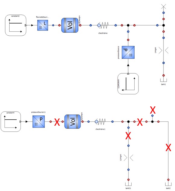
The general rule to follow is: always connect a RED port with a BLUE one, alternating capacitive/resistive. From each hydraulic port can start maximum 1 line: for more connections use hydraulic nodes.

RED = capacitive element
BLUE = resistive element

Do not connect two elements of the same type to each other (e.g., two volumes)

RED pin - BLUE pin rule

Always connect a RED port with a BLUE one.

Some elements do not have ports of the same type, for example the hydraulic node always has 1 RED port and ≥1 BLUE. These are elements that are neither resistive nor capacitive, but simple passage, measurement, transformation or connection elements.

Hydraulic connections

Why is the distinction of two component types important?

Capacitive elements are designed to process the balance of volumetric flow rate entering/exiting and process the pressure through the bulk modulus equation.

Resistive elements, on the other hand, receive pressure from the interface pins and process the volumetric flow rate passing through in relation to the pressure drop.

All flow rates are corrected by the factor ρ₀/ρ (reference density vs. current density) - In-depth

FluidProp

The FluidProp model defines the properties of the fluid used in the simulation. Inside it, it is possible to characterize up to 3 distinct fluids. Each simulation element that interfaces with a fluid (for example a valve) has the fluid_index parameter, whose value indicates which of the three fluids interacts with the object. In this way, it is possible to create simulation circuits with components that use different fluids.

FluidProp

When this model is instantiated, it cannot be given a custom name, but must keep its original name fluidProp and must never be renamed. (1)

as a consequence, there cannot be more than one object of this type in the same environment. No more than 3 fluids can be characterized!

Same fluid for every connection

Normally, all hydraulic components with ports connected to each other should have the same fluid index.

An exception to this rule could be the case where two different fluids are used to simulate oil at different temperatures. In this case, by changing the fluid index, one component can receive cold oil and the next one hot oil. It is up to the simulator to decide on which criterion to use these properties.

Structure

Among the fluid types, it is possible to choose from a few already-configured fluid presets:

Fluid_A: Industrial oil ISO-VG 46 with 0.1% air by volume
Fluid_B: Industrial oil ISO-VG 32 with 0.1% air by volume
Fluid_C: Industrial oil ISO-VG 46 with 0.5% air by volume
Water: water with 0.5% air by volume

alternatively, it is possible to select Custom to enter custom properties.

FluidProp page

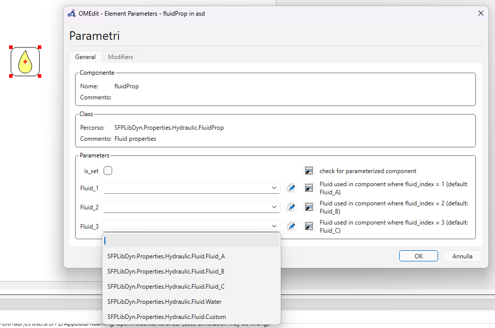
Using the edit button icon , the parameterization page for each fluid opens.

Fluid page

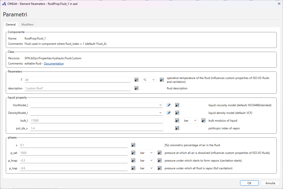
Within this window it is possible to modify the main properties, as well as choose the calculation models for density and viscosity: the drop-down menu allows the model to be selected, while the edit button allows the parameterization page of the chosen model to be opened. Each window has a hyperlink that opens the documentation page related to that model.

The choice of these sub-models affects only the calculations of the liquid component (while the vapor and gas parts have a fixed model). For completeness, the available models are listed below. The following table shows a summary of the calculation dependencies on the independent variables, followed by a detailed description of each individual model.

Property	Model	p	When to use it
Viscosity	Constant		If you want to use a precise viscosity value
Viscosity	ISO3448		Class from ISO VG, for applications with controlled pressure values
Viscosity	ISO3448Extended		If you want to use a standard oil for high-pressure applications
Viscosity	LambdaExtended		Fully characterized fluid, if the sensitivity terms are known (or experimental results for 3 distinct conditions are available)
Density	Constant	*	If you want to use a precise viscosity value
Density	GeneralExpansionCoeff	*	With mineral oils with a known expansion coefficient
Density	VCF	*	Draws on the standards most widely used in the petroleum industry, so that the data reported on suppliers' technical data sheets can be used directly.

(*) The dependence of density on local pressure is always present, regardless of the selected model. All models in fact require the bulk modulus, used by the library's equations to describe the compressibility of the fluid. The density models act exclusively on the variation with temperature.

Viscosity calculation models

Constant: keeps the kinematic viscosity constant for the entire simulation;
ISO3448: allows an oil to be chosen based on the standard. Viscosity is calculated as the fluid temperature varies;
ISO3448Extended: like the previous model, but a correction coefficient is introduced as a function of local pressure (locally variable for each hydraulic element)
LambdaExtended: uses correction coefficients to vary viscosity as a function of fluid temperature and local pressure

The Constant model is suggested if you want to shorten the simulation time, since the calculation models will be simpler. The more advanced models, on the other hand, are recommended for more accurate results, especially for solutions that reach high pressures, where the contribution of pressure raises viscosity values in a non-negligible way.

Density calculation models

Constant: the density of the liquid remains constant as the fluid temperature varies
GeneralExpansionCoeff: a generic expansion model is used as temperature increases
VCF: a correct calculation model, widely used in the industrial sector for petroleum liquids, is provided

Unlike the viscosity calculation models, the density calculation always depends on local pressure (this would not be an acceptable simplification and would result in a constant compressibility modulus).

Volumetric flow rate correction

Each volumetric flow rate value is corrected by the factor ρ₀/ρ (reference density over current density). This means that when we observe a flow rate value crossing a pin, we are actually observing a mass flow masked as volumetric flow rate. In fact, dividing the real volumetric flow rate by the density ρ we obtain the mass flow rate which, through the mass conservation equation, guarantees the continuity of matter. Only to have results in a volumetric quantity we multiply by ρ₀, density at T = 15.6°C and atmospheric pressure - ASTM standard.

This corrective value is ~1 for most cases; it assumes a value significantly ≠ 1 in cavitation phases. If a pump were to cavitate, thanks to the convention used we would see a very low suction flow rate, while in reality a volumetric pump, by definition, always displaces the same volume amount. The difference lies in the density of the sucked material: during cavitation the fluid has a much lower density than expected, because it is composed of a portion of gas.

Example file: cavitation

model cavitazione
SFPLibDyn.Hydraulic.Sources.Pumps.FixedUniDirPump fixedUniDirPump(max_displ = 1.6e-4)  annotation(
    Placement(transformation(origin = {2, 22}, extent = {{-15, -15}, {15, 15}})));
SFPLibDyn.Mechanical.Rotational.Sources.Motor motor annotation(
    Placement(transformation(origin = {-42, 22}, extent = {{-15, -15}, {15, 15}})));
SFPLibDyn.Signals.Source.Constant constant1(k = 1000)  annotation(
    Placement(transformation(origin = {-76, 22}, extent = {{-10, -10}, {10, 10}})));
SFPLibDyn.Hydraulic.Sources.Tank tank annotation(
    Placement(transformation(origin = {42, 40}, extent = {{-6, -4.5}, {6, 4.5}})));
SFPLibDyn.Hydraulic.Volumes.Volume2p volume2p(vol_0 = 0.001, pressure(start = 0, fixed = true))  annotation(
    Placement(transformation(origin = {2, -14}, extent = {{-10, -10}, {10, 10}})));
SFPLibDyn.Hydraulic.Orifices.OrificeVariable orificeVariable(min_signal = 0.01, diam = 0.036)  annotation(
    Placement(transformation(origin = {2, -45}, extent = {{-6, -12}, {6, 12}})));
SFPLibDyn.Hydraulic.Sources.Tank tank1 annotation(
    Placement(transformation(origin = {2, -70}, extent = {{-6, -4.5}, {6, 4.5}})));
SFPLibDyn.Signals.Source.Ramp ramp(val_initial = 1, slope = -1, time_start = 0.2)  annotation(
    Placement(transformation(origin = {-26, -52}, extent = {{-10, -10}, {10, 10}})));
equation
connect(fixedUniDirPump.r1, motor.r1) annotation(
    Line(points = {{-16, 22}, {-24, 22}}));
connect(motor.u1, constant1.y1) annotation(
    Line(points = {{-56, 22}, {-66, 22}}));
connect(tank.h1, fixedUniDirPump.h2) annotation(
    Line(points = {{42, 44}, {42, 60}, {2, 60}, {2, 38}}));
connect(fixedUniDirPump.h1, volume2p.h2) annotation(
    Line(points = {{2, 8}, {2, -4}}));
connect(volume2p.h1, orificeVariable.h2) annotation(
    Line(points = {{2, -24}, {2, -33}}));
connect(orificeVariable.h1, tank1.h1) annotation(
    Line(points = {{2, -57}, {2, -66}}));
connect(orificeVariable.u1, ramp.y1) annotation(
    Line(points = {{-2.5, -52}, {-16, -52}}));

annotation(
    uses(SFPLibDyn(version = "3.2")),
Diagram(coordinateSystem(extent = {{-100, -100}, {100, 100}}, grid = {1, 1})),
version = "",
__OpenModelica_simulationFlags(lv = "LOG_STDOUT,LOG_ASSERT,LOG_STATS", s = "dassl", variableFilter = ".*"),
experiment(StartTime = 0, StopTime = 2, Tolerance = 1e-06, Interval = 0.0004));
end cavitazione;